# defining murder rate as before
murder_rate <- murders$total / murders$population * 100000
# creating a logical vector that specifies if the murder rate in that state is less than or equal to 0.71
index <- murder_rate <= 0.71
# determining which states have murder rates less than or equal to 0.71
murders$state[index]
# calculating how many states have a murder rate less than or equal to 0.71
sum(index)

# creating the two logical vectors representing our conditions
west <- murders$region == "West"
safe <- murder_rate <= 1
# defining an index and identifying states with both conditions true
index <- safe & west
murders$state[index]Indexing, Data Wrangling, Plots
In this section, I will introduce the R commands and techniques that help you wrangle, analyze, and visualize data.
In Indexing, you will: - Subset a vector based on properties of another vector.
Use multiple logical operators to index vectors.
Extract the indices of vector elements satisfying one or more logical conditions.
Extract the indices of vector elements matching with another vector.
Determine which elements in one vector are present in another vector.
In basic data wrangling, you will:
Wrangle data tables using functions in the dplyr package.
Modify a data table by adding or changing columns.
Subset rows in a data table.
Subset columns in a data table.
Perform a series of operations using the pipe operator.
Create data frames.
In basic plots, you will: - Plot data in scatter plots, box plots, and histograms.
In summarizing with dplyr, you will: - Use summarize() to facilitate summarizing data in dplyr.
Learn about the dot placeholder.
Learn how to group and then summarize in dplyr.
Learn how to sort data tables in dplyr.
In the rest section, you will: - Learn how to subset and summarize data using data.table.
- Learn how to sort data frames using data.table.
Indexing
Key Point
We can use logicals to index vectors.
Using the function sum()on a logical vector returns the number of entries that are true.
The logical operator “&” makes two logicals true only when they are both true.
Code
Indexing Functions
Key Points
Code
x <- c(FALSE, TRUE, FALSE, TRUE, TRUE, FALSE)
which(x)    # returns indices that are TRUE

# to determine the murder rate in Massachusetts we may do the following
index <- which(murders$state == "Massachusetts")
index
murder_rate[index]

# to obtain the indices and subsequent murder rates of New York, Florida, Texas, we do:
index <- match(c("New York", "Florida", "Texas"), murders$state)
index
murders$state[index]
murder_rate[index]

x <- c("a", "b", "c", "d", "e")
y <- c("a", "d", "f")
y %in% x

# to see if Boston, Dakota, and Washington are states
c("Boston", "Dakota", "Washington") %in% murders$state
Basic Data Wrangling
Key Points
To change a data table by adding a new column, or changing an existing one, we use the
mutate()function.To filter the data by subsetting rows, we use the function
filter().To subset the data by selecting specific columns, we use the
select()function.We can perform a series of operations by sending the results of one function to another function using the pipe operator,
%>%.
Creating Data Frames
Note
The default settings in R have changed as of version 4.0, and it is no longer necessary to include the code stringsAsFactors = FALSE in order to keep strings as characters. Putting the entries in quotes, as in the example, is adequate to keep strings as characters. The stringsAsFactors = FALSE code is useful in certain other situations, but you do not need to include it when you create data frames in this manner.
Key Points
We can use the
data.frame()function to create data frames.Formerly, the
data.frame()function turned characters into factors by default. To avoid this, we could utilize thestringsAsFactorsargument and set it equal to false. As of R 4.0, it is no longer necessary to include thestringsAsFactorsargument, because R no longer turns characters into factors by default.
Code
# creating a data frame with stringAsFactors = FALSE
grades <- data.frame(names = c("John", "Juan", "Jean", "Yao"),
                     exam_1 = c(95, 80, 90, 85),
                     exam_2 = c(90, 85, 85, 90),
                     stringsAsFactors = FALSE)
Basic Plots
Key Points
We can create a simple scatterplot using the function
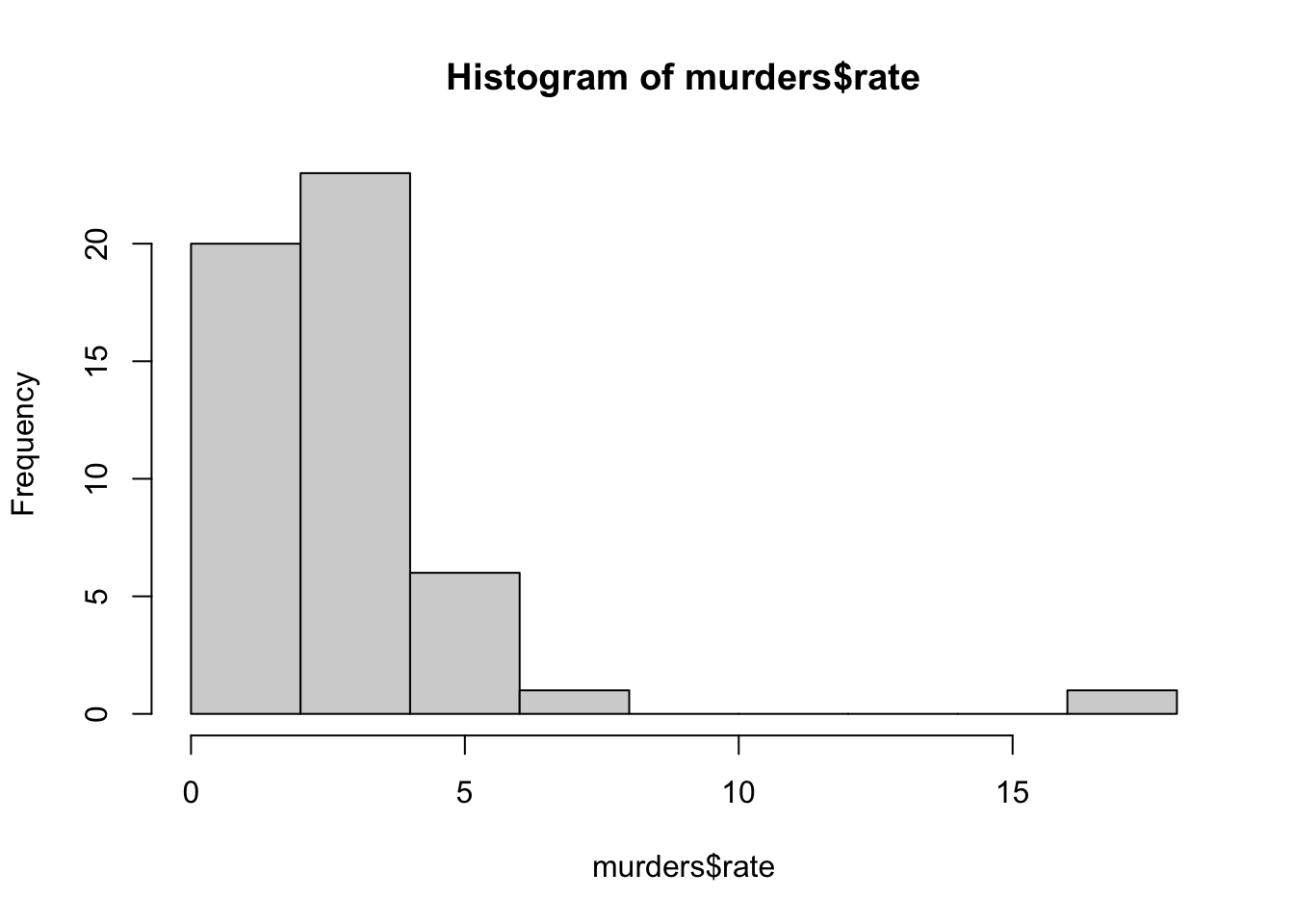
plot().Histograms are graphical summaries that give you a general overview of the types of values you have. In R, they can be produced using the
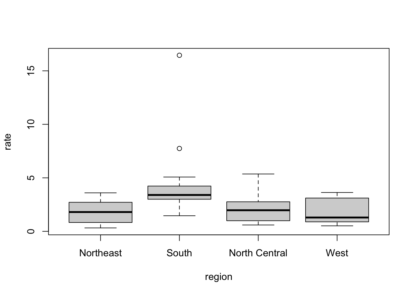
hist()function.Boxplots provide a more compact summary of a distribution than a histogram and are more useful for comparing distributions. They can be produced using the
boxplot()function.
Code
# a simple scatterplot of total murders versus population
x <- murders$population /10^6
y <- murders$total
plot(x, y)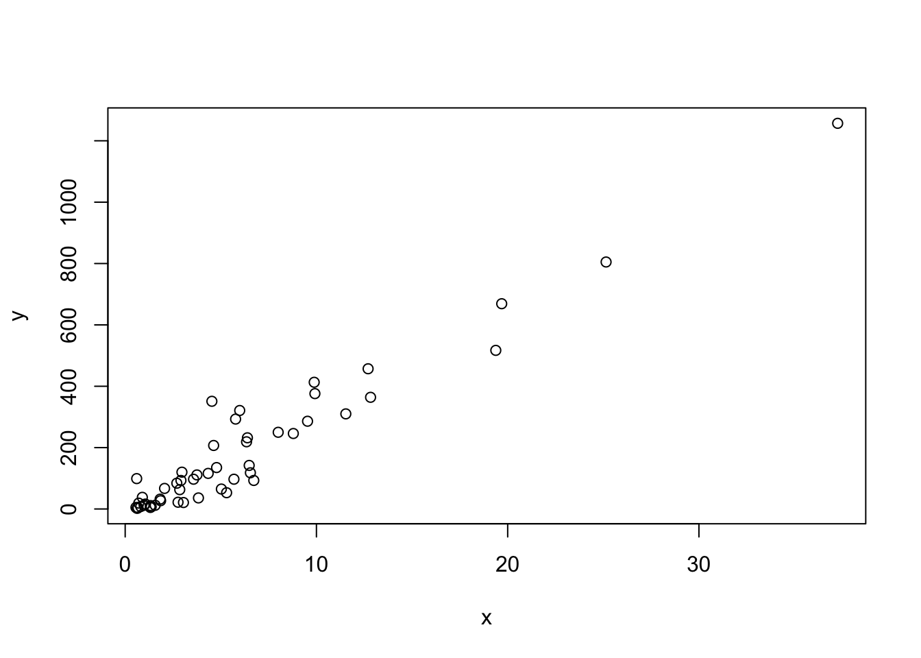
The summarize function
Key Points
Summarizing data is an important part of data analysis.
Some summary ststistics are the mean, median, and standard deviation.
The
summarize()function from dplyr provides an easy way to compute summary statics.
Code
# minimum, median, and maximum murder rate for the states in the West region
s <- murders %>%
  filter(region == "West") %>%
  summarize(minimum = min(rate),
            median = median(rate),
            maximum = max(rate))
s
minimum median maximum
1 0.514592 1.292453 3.629527# accessing the components with the accessor $
s$median[1] 1.292453s$maximum[1] 3.629527# average rate unadjusted by population size
mean(murders$rate)[1] 2.779125# average rate adjusted by population size
us_murder_rate <- murders %>%
summarize(rate = sum(total) / sum(population) * 10^5)
us_murder_rate rate
1 3.034555Summarizing with more than one value
Key Points
- The
quantile()function can be used to return the min, median, and max in a single line of code.
Code
# minimum, median, and maximum murder rate for the states in the West region using quantile
# note that this returns a vector
murders %>%
filter(region == "West") %>%
summarize(range = quantile(rate, c(0, 0.5, 1)))Warning: Returning more (or less) than 1 row per `summarise()` group was deprecated in
dplyr 1.1.0.
ℹ Please use `reframe()` instead.
ℹ When switching from `summarise()` to `reframe()`, remember that `reframe()`
always returns an ungrouped data frame and adjust accordingly. range
1 0.514592
2 1.292453
3 3.629527# returning minimum, median, and maximum as a data frame
my_quantile <- function(x){
r <- quantile(x, c(0, 0.5, 1))
data.frame(minimum = r[1], median = r[2], maximum = r[3])
}
murders %>%
filter(region == "West") %>%
summarize(my_quantile(rate)) minimum median maximum
1 0.514592 1.292453 3.629527Pull to access to columns
Key Points
Code
# average rate adjusted by population size
us_murder_rate <- murders %>%
  summarize(rate = sum(total) / sum(population) * 10^5)
us_murder_rate
rate
1 3.034555# us_murder_rate is stored as a data frame
class(us_murder_rate)[1] "data.frame"[1] 3.034555# using pull to save the number directly
us_murder_rate <- murders %>%
summarize(rate = sum(total) / sum(population) * 10^5) %>%
pull(rate)
us_murder_rate[1] 3.034555# us_murder_rate is now stored as a number
class(us_murder_rate)[1] "numeric"The dot placeholder
Key Points
- The
dot (.)can be thought of as a placeholder for the data being passed through the pipe.
# average rate adjusted by population size
us_murder_rate <- murders %>%
  summarize(rate = sum(total) / sum(population) * 10^5)
us_murder_rate
rate
1 3.034555# using the dot to access the rate
us_murder_rate <- murders %>%
summarize(rate = sum(total) / sum(population) * 10^5) %>%
.$rate
us_murder_rate[1] 3.034555class(us_murder_rate)[1] "numeric"Group then summarize
Key Points
Splitting data into groups and then computing summaries for each group is a common operation in data exploration.
We can use the dplyr
group_by()function to create a special grouped data frame to facilitate such summaries.
# A tibble: 51 × 6
# Groups:   region [4]
   state                abb   region    population total  rate
   <chr>                <chr> <fct>          <dbl> <dbl> <dbl>
 1 Alabama              AL    South        4779736   135  2.82
 2 Alaska               AK    West          710231    19  2.68
 3 Arizona              AZ    West         6392017   232  3.63
 4 Arkansas             AR    South        2915918    93  3.19
 5 California           CA    West        37253956  1257  3.37
 6 Colorado             CO    West         5029196    65  1.29
 7 Connecticut          CT    Northeast    3574097    97  2.71
 8 Delaware             DE    South         897934    38  4.23
 9 District of Columbia DC    South         601723    99 16.5
10 Florida              FL    South       19687653   669  3.40
# ℹ 41 more rows
# A tibble: 4 × 2
region median
<fct> <dbl>
1 Northeast 1.80
2 South 3.40
3 North Central 1.97
4 West 1.29Sorting data tables
Key Points
Code
                 state abb        region population total       rate
1              Wyoming  WY          West     563626     5  0.8871131
2 District of Columbia  DC         South     601723    99 16.4527532
3              Vermont  VT     Northeast     625741     2  0.3196211
4         North Dakota  ND North Central     672591     4  0.5947151
5               Alaska  AK          West     710231    19  2.6751860
6         South Dakota  SD North Central     814180     8  0.9825837
# order the states by murder rate - the default is ascending order
murders %>% arrange(rate) %>% head() state abb region population total rate
1 Vermont VT Northeast 625741 2 0.3196211
2 New Hampshire NH Northeast 1316470 5 0.3798036
3 Hawaii HI West 1360301 7 0.5145920
4 North Dakota ND North Central 672591 4 0.5947151
5 Iowa IA North Central 3046355 21 0.6893484
6 Idaho ID West 1567582 12 0.7655102 state abb region population total rate
1 District of Columbia DC South 601723 99 16.452753
2 Louisiana LA South 4533372 351 7.742581
3 Missouri MO North Central 5988927 321 5.359892
4 Maryland MD South 5773552 293 5.074866
5 South Carolina SC South 4625364 207 4.475323
6 Delaware DE South 897934 38 4.231937# order the states by region and then by murder rate within region
murders %>% arrange(region, rate) %>% head() state abb region population total rate
1 Vermont VT Northeast 625741 2 0.3196211
2 New Hampshire NH Northeast 1316470 5 0.3798036
3 Maine ME Northeast 1328361 11 0.8280881
4 Rhode Island RI Northeast 1052567 16 1.5200933
5 Massachusetts MA Northeast 6547629 118 1.8021791
6 New York NY Northeast 19378102 517 2.6679599 state abb region population total rate
1 Arizona AZ West 6392017 232 3.629527
2 Delaware DE South 897934 38 4.231937
3 District of Columbia DC South 601723 99 16.452753
4 Georgia GA South 9920000 376 3.790323
5 Louisiana LA South 4533372 351 7.742581
6 Maryland MD South 5773552 293 5.074866
7 Michigan MI North Central 9883640 413 4.178622
8 Mississippi MS South 2967297 120 4.044085
9 Missouri MO North Central 5988927 321 5.359892
10 South Carolina SC South 4625364 207 4.475323# return the top 10 states ranked by murder rate, sorted by murder rate
murders %>% arrange(desc(rate)) %>% top_n(10)Selecting by rate state abb region population total rate
1 District of Columbia DC South 601723 99 16.452753
2 Louisiana LA South 4533372 351 7.742581
3 Missouri MO North Central 5988927 321 5.359892
4 Maryland MD South 5773552 293 5.074866
5 South Carolina SC South 4625364 207 4.475323
6 Delaware DE South 897934 38 4.231937
7 Michigan MI North Central 9883640 413 4.178622
8 Mississippi MS South 2967297 120 4.044085
9 Georgia GA South 9920000 376 3.790323
10 Arizona AZ West 6392017 232 3.629527Introduction to data.table
Key Points
In this course, we often use tidyverse packages to illustrate because these packages tend to have code that is very readable for beginners.
There are other approaches to wrangling and analyzing data in R that are faster and better at handling large objects, such as the data.table package.
Selecting in data.table uses notation similar to that used with matrices.
To add a column in data.table, you can use the := function.
Because the data.table package is designed to avoid wasting memory, when you make a copy of a table, it does not create a new object. The := function changes by reference. If you want to make an actual copy, you need to use the copy() function.
Side note: the R language has a new, built-in pipe operator as of version 4.1: |>. This works similarly to the pipe %>% you are already familiar with. You can read more about the |> pipe here External link.
Code
# install the data.table package before you use it!
install.packages("data.table")

# load data.table package
library(data.table)

# load other packages and datasets
library(tidyverse)
library(dplyr)
library(dslabs)
data(murders)

# convert the data frame into a data.table object
murders <- setDT(murders)

# selecting in dplyr
select(murders, state, region)

# selecting in data.table - 2 methods
murders[, c("state", "region")] |> head()
murders[, .(state, region)] |> head()

# adding or changing a column in dplyr
murders <- mutate(murders, rate = total / population * 10^5)

# adding or changing a column in data.table
murders[, rate := total / population * 100000]
head(murders)
murders[, ":="(rate = total / population * 100000, rank = rank(population))]

# y is referring to x and := changes by reference
x <- data.table(a = 1)
y <- x

x[,a := 2]
y

y[,a := 1]
x

# use copy to make an actual copy
x <- data.table(a = 1)
y <- copy(x)
x[,a := 2]
y
Subsetting with data.table
Key Points
Subsetting in data.table uses notation similar to that used with matrices.
Code
# load packages and prepare the data
library(tidyverse)
library(dplyr)
library(dslabs)
data(murders)
library(data.table)
murders <- setDT(murders)
murders <- mutate(murders, rate = total / population * 10^5)
murders[, rate := total / population * 100000]

# subsetting in dplyr
filter(murders, rate <= 0.7)

# subsetting in data.table
murders[rate <= 0.7]

# combining filter and select in data.table
murders[rate <= 0.7, .(state, rate)]

# combining filter and select in dplyr
murders %>% filter(rate <= 0.7) %>% select(state, rate)
Summarizing with data.table
Key Points
In data.table we can call functions inside
.()and they will be applied to rows.The
group_byfollowed by summarize in dplyr is performed in one line in data.table using the by argument.
Code
# load packages and prepare the data - heights dataset
library(tidyverse)
library(dplyr)
library(dslabs)
data(heights)
heights <- setDT(heights)

# summarizing in dplyr
s <- heights %>%
  summarize(average = mean(height), standard_deviation = sd(height))

# summarizing in data.table
s <- heights[, .(average = mean(height), standard_deviation = sd(height))]

# subsetting and then summarizing in dplyr
s <- heights %>%
  filter(sex == "Female") %>%
  summarize(average = mean(height), standard_deviation = sd(height))

# subsetting and then summarizing in data.table
s <- heights[sex == "Female", .(average = mean(height), standard_deviation = sd(height))]

# previously defined function
median_min_max <- function(x){
  qs <- quantile(x, c(0.5, 0, 1))
  data.frame(median = qs[1], minimum = qs[2], maximum = qs[3])
}

# multiple summaries in data.table
heights[, .(median_min_max(height))]

# grouping then summarizing in data.table
heights[, .(average = mean(height), standard_deviation = sd(height)), by = sex]
Sorting data frames
Key Points
To order rows in a data frame using data.table, we can use the same approach we used for filtering.
The default sort is an ascending order, but we can also sort tables in descending order.
We can also perform nested sorting by including multiple variables in the desired sort order.
Code
# load packages and datasets and prepare the data
library(tidyverse)
library(dplyr)
library(data.table)
library(dslabs)
data(murders)
murders <- setDT(murders)
murders[, rate := total / population * 100000]

# order by population
murders[order(population)] |> head()

# order by population in descending order
murders[order(population, decreasing = TRUE)]

# order by region and then murder rate
murders[order(region, rate)]